The Methylome in Female Adolescent Conduct Disorder: Neural Pathomechanisms and Environmental Risk Factors
Preprocessing
AG Chiocchetti
29 Dezember 2020
Last updated: 2021-09-24
Checks: 7 0
Knit directory: femNATCD_MethSeq/
This reproducible R Markdown analysis was created with workflowr (version 1.6.2). The Checks tab describes the reproducibility checks that were applied when the results were created. The Past versions tab lists the development history.
Great! Since the R Markdown file has been committed to the Git repository, you know the exact version of the code that produced these results.
Great job! The global environment was empty. Objects defined in the global environment can affect the analysis in your R Markdown file in unknown ways. For reproduciblity it’s best to always run the code in an empty environment.
The command set.seed(20210128) was run prior to running the code in the R Markdown file. Setting a seed ensures that any results that rely on randomness, e.g. subsampling or permutations, are reproducible.
Great job! Recording the operating system, R version, and package versions is critical for reproducibility.
Nice! There were no cached chunks for this analysis, so you can be confident that you successfully produced the results during this run.
Great job! Using relative paths to the files within your workflowr project makes it easier to run your code on other machines.
Great! You are using Git for version control. Tracking code development and connecting the code version to the results is critical for reproducibility.
The results in this page were generated with repository version 56bb68f. See the Past versions tab to see a history of the changes made to the R Markdown and HTML files.
Note that you need to be careful to ensure that all relevant files for the analysis have been committed to Git prior to generating the results (you can use wflow_publish or wflow_git_commit). workflowr only checks the R Markdown file, but you know if there are other scripts or data files that it depends on. Below is the status of the Git repository when the results were generated:
Ignored files:
    Ignored:    .Rhistory
    Ignored:    .Rproj.user/
    Ignored:    analysis/.Rhistory
    Ignored:    code/.Rhistory
    Ignored:    data/Epicounts.csv
    Ignored:    data/Epimeta.csv
    Ignored:    data/Epitpm.csv
    Ignored:    data/KangUnivers.txt
    Ignored:    data/Kang_DataPreprocessing.RData
    Ignored:    data/Kang_dataset_genesMod_version2.txt
    Ignored:    data/PatMeta.csv
    Ignored:    data/ProcessedData.RData
    Ignored:    data/RTrawdata/
    Ignored:    data/SNPCommonFilt.csv
    Ignored:    data/femNAT_PC20.txt
    Ignored:    output/BrainMod_Enrichemnt.pdf
    Ignored:    output/Brain_Module_Heatmap.pdf
    Ignored:    output/DMR_Results.csv
    Ignored:    output/GOres.xlsx
    Ignored:    output/LME_GOplot.pdf
    Ignored:    output/LME_Results.csv
    Ignored:    output/LME_Results_Sig.csv
    Ignored:    output/LME_tophit.svg
    Ignored:    output/ProcessedData.RData
    Ignored:    output/RNAvsMETplots.pdf
    Ignored:    output/Regions_GOplot.pdf
    Ignored:    output/ResultsgroupComp.txt
    Ignored:    output/SEM_summary_groupEpi_M15.txt
    Ignored:    output/SEM_summary_groupEpi_M2.txt
    Ignored:    output/SEM_summary_groupEpi_M_all.txt
    Ignored:    output/SEM_summary_groupEpi_TopHit.txt
    Ignored:    output/SEM_summary_groupEpi_all.txt
    Ignored:    output/SEMplot_Epi_M15.html
    Ignored:    output/SEMplot_Epi_M15.png
    Ignored:    output/SEMplot_Epi_M15_files/
    Ignored:    output/SEMplot_Epi_M2.html
    Ignored:    output/SEMplot_Epi_M2.png
    Ignored:    output/SEMplot_Epi_M2_files/
    Ignored:    output/SEMplot_Epi_M_all.html
    Ignored:    output/SEMplot_Epi_M_all.png
    Ignored:    output/SEMplot_Epi_M_all_files/
    Ignored:    output/SEMplot_Epi_TopHit.html
    Ignored:    output/SEMplot_Epi_TopHit.png
    Ignored:    output/SEMplot_Epi_TopHit_files/
    Ignored:    output/SEMplot_Epi_all.html
    Ignored:    output/SEMplot_Epi_all.png
    Ignored:    output/SEMplot_Epi_all_files/
    Ignored:    output/barplots.pdf
    Ignored:    output/circos_DMR_tags.svg
    Ignored:    output/circos_LME_tags.svg
    Ignored:    output/clinFact.RData
    Ignored:    output/dds_filt_analyzed.RData
    Ignored:    output/designh0.RData
    Ignored:    output/designh1.RData
    Ignored:    output/envFact.RData
    Ignored:    output/functional_Enrichemnt.pdf
    Ignored:    output/gostres.pdf
    Ignored:    output/modelFact.RData
    Ignored:    output/resdmr.RData
    Ignored:    output/resultsdmr_table.RData
    Ignored:    output/table1_filtered.Rmd
    Ignored:    output/table1_filtered.docx
    Ignored:    output/table1_unfiltered.Rmd
    Ignored:    output/table1_unfiltered.docx
    Ignored:    setup_built.R
Note that any generated files, e.g. HTML, png, CSS, etc., are not included in this status report because it is ok for generated content to have uncommitted changes.
These are the previous versions of the repository in which changes were made to the R Markdown (analysis/01_Preprocessing.Rmd) and HTML (docs/01_Preprocessing.html) files. If you’ve configured a remote Git repository (see ?wflow_git_remote), click on the hyperlinks in the table below to view the files as they were in that past version.
| File | Version | Author | Date | Message |
|---|---|---|---|---|
| html | 43333cc | achiocch | 2021-09-24 | adds new build |
| html | b497cc9 | achiocch | 2021-09-17 | Build site. |
| html | ccbc9e4 | achiocch | 2021-08-10 | Build site. |
| html | 70cd649 | achiocch | 2021-08-06 | Build site. |
| html | 2a53a87 | achiocch | 2021-08-06 | Build site. |
| html | e3a9ae3 | achiocch | 2021-08-04 | Build site. |
| html | f6bbdc0 | achiocch | 2021-08-04 | Build site. |
| html | 710904a | achiocch | 2021-08-03 | Build site. |
| html | 16112c3 | achiocch | 2021-08-03 | wflow_publish(c(“analysis/", "code/”, “docs/”)) |
| html | cde8384 | achiocch | 2021-08-03 | Build site. |
| html | d761be4 | achiocch | 2021-07-31 | Build site. |
| html | b452d2f | achiocch | 2021-07-30 | wflow_publish(c(“analysis/", "code/”, "docs/*")) |
| Rmd | 1a9f36f | achiocch | 2021-07-30 | reviewed analysis |
| html | 2734c4e | achiocch | 2021-05-08 | Build site. |
| Rmd | a847823 | achiocch | 2021-05-08 | wflow_publish(c(“analysis/", "code/”, "docs/*")) |
| html | a847823 | achiocch | 2021-05-08 | wflow_publish(c(“analysis/", "code/”, "docs/*")) |
| html | 9cc52f7 | achiocch | 2021-05-08 | Build site. |
| Rmd | 158d0b4 | achiocch | 2021-05-08 | wflow_publish(c(“analysis/", "code/”, "docs/*")) |
| html | 158d0b4 | achiocch | 2021-05-08 | wflow_publish(c(“analysis/", "code/”, "docs/*")) |
| html | 0f262d1 | achiocch | 2021-05-07 | Build site. |
| html | 5167b90 | achiocch | 2021-05-07 | wflow_publish(c(“analysis/", "code/”, "docs/*")) |
| Rmd | b5b9b9f | achiocch | 2021-05-07 | maual commit |
| html | b5b9b9f | achiocch | 2021-05-07 | maual commit |
| html | 05aac7f | achiocch | 2021-04-23 | Build site. |
| html | f5c5265 | achiocch | 2021-04-19 | Build site. |
| html | 17f1eec | achiocch | 2021-04-10 | Build site. |
| html | 91de221 | achiocch | 2021-04-05 | Build site. |
| Rmd | acd87d4 | achiocch | 2021-04-05 | wflow_publish(c(“analysis/", "code/”, "docs/*")) |
| Rmd | b6c6b33 | achiocch | 2021-04-05 | updated GO function, and model def |
| html | 4ea1bba | achiocch | 2021-02-25 | Build site. |
| Rmd | 6c21638 | achiocch | 2021-02-25 | wflow_publish(c(“analysis/", "code/”, "docs/*"), update = F) |
| html | 6c21638 | achiocch | 2021-02-25 | wflow_publish(c(“analysis/", "code/”, "docs/*"), update = F) |
source(paste0(Home,"/code/custom_functions.R"))Lade nötiges Paket: RCircosLade nötiges Paket: scales
Attache Paket: 'scales'The following object is masked from 'package:purrr':
discardThe following object is masked from 'package:readr':
col_factorInitializing rawdata
## load Data  ####
EpiData = fread(paste0(Home,"/data/Epicounts.csv"), header = T, data.table=F)
EpiData = EpiData %>% column_to_rownames("ID")

EpiMeta = fread(paste0(Home,"/data/Epimeta.csv"), header = T, data.table=F)
EpiMeta = EpiMeta %>% column_to_rownames("ID")

Patdata = fread(paste0(Home,"/data/PatMeta.csv"), header = T, data.table=F)
Patdata = Patdata %>% column_to_rownames("V1")

SNPdata = fread(paste0(Home,"/data/SNPCommonFilt.csv"), header = T, data.table=F)
SNPdata = SNPdata %>% column_to_rownames("V1")

PopPCAdata = fread(paste0(Home,"/data/femNAT_PC20.txt"), header = T, data.table=F)
PopPCAdata$ID = paste0("ID_", gsub("-", "_", PopPCAdata$FID))
PopPCAdata = PopPCAdata %>% column_to_rownames("ID")
PopPCAdata = PopPCAdata[rownames(Patdata), grepl("PC_",colnames(PopPCAdata))]

Patdata = cbind(Patdata, PopPCAdata)
Patdata$group = factor(Patdata$group, c(0,1), c("CTRL", "CD"))
Patdata$group = relevel(Patdata$group, "CTRL")

Patdata$Age = Patdata$Alter

Patdata$site = factor(substr(Patdata$ID_femNAT, 1,2),
                      c("01","02", "10", "11", "12"), c("FRA", "AAC", "BCN", "BLB", "SZG"))

Patdata$Pubstat = as.factor(gsub(" ", "", Patdata$Pubstat))

Patdata$contraceptives = yesnofac(Patdata$contraceptives)
Patdata$Ever_smoked = factor(Patdata$Ever_smoked, c(0, 1,2), c(NA, "no", "yes"))


allowedvalues=as.character(c(0,1,8, NA))


for (i in 1:ncol(Patdata)) {
  if(sum(Patdata[,i] %in% allowedvalues)==nrow(Patdata)){
    Patdata[,i] = yesnofac(Patdata[,i])
    print(colnames(Patdata)[i])
  }

}
[1] "smoke"
[1] "drugs"
[1] "aggress"
[1] "stress"
[1] "mpsych_4_12"
[1] "mpsych_gt12"
[1] "ppsych_le12"
[1] "inconsist"
[1] "single"
[1] "disharm"
[1] "isolation"
[1] "psych_fam"
[1] "Dep_life"
[1] "anp_life"
[1] "CD_life"
[1] "ADHD_life"
[1] "TIC_life"
[1] "ODD_life"
[1] "DMDD_life"
[1] "Alk_life"
[1] "SUD_life"
[1] "Anx_life"
[1] "OCD_life"
[1] "PTSD_life"
[1] "Elim_life"
[1] "Eat_life"
[1] "Oth_life"
[1] "Bip_life"
[1] "Scz_life"
[1] "medication"SNPdatafilt = SNPdata[complete.cases(SNPdata),]
display_tab(head(EpiMeta))| CHR | start | stop | gene | feature | cpg | tf_binding | raw_gene | distance | samples_per_target | mean | std | |
|---|---|---|---|---|---|---|---|---|---|---|---|---|
| chr1+_10482_10487 | 1 | 10482 | 10487 | DDX11L1 | upstream | NoCpg | TAF7_(SQ-8)//ZBTB33 | DDX11L1 | 0 | 100 | 20.569 | 13.877 |
| chr1+_10495_10500 | 1 | 10495 | 10500 | DDX11L1 | upstream | NoCpg | TAF7_(SQ-8)//ZBTB33 | DDX11L1 | 0 | 98 | 10.608 | 9.030 |
| chr1+_10587_10592 | 1 | 10587 | 10592 | DDX11L1 | upstream | NoCpg | DDX11L1 | 0 | 85 | 6.176 | 6.170 | |
| chr1+_10639_10644 | 1 | 10639 | 10644 | DDX11L1 | upstream | NoCpg | DDX11L1 | 0 | 54 | 0.941 | 1.241 | |
| chr1+_10668_10673 | 1 | 10668 | 10673 | DDX11L1 | upstream | NoCpg | DDX11L1 | 0 | 51 | 0.922 | 1.272 | |
| chr1+_10697_10702 | 1 | 10697 | 10702 | DDX11L1 | upstream | NoCpg | DDX11L1 | 0 | 65 | 1.029 | 1.085 |
display_tab(head(EpiData))| ID_01_0023 | ID_01_0028 | ID_01_0029 | ID_01_0056 | ID_01_0074 | ID_01_0075 | ID_01_0145 | ID_01_0173 | ID_01_0185 | ID_01_0209 | ID_01_0221 | ID_01_0248 | ID_01_0249 | ID_01_0260 | ID_01_0284 | ID_01_0286 | ID_01_0289 | ID_01_0292 | ID_01_0293 | ID_01_0294 | ID_01_0295 | ID_01_0311 | ID_01_0322 | ID_01_0325 | ID_01_0343 | ID_01_0362 | ID_01_0365 | ID_01_0379 | ID_01_0382 | ID_01_0383 | ID_01_0385 | ID_01_0386 | ID_01_0400 | ID_01_0431 | ID_01_0433 | ID_01_0439 | ID_01_0500 | ID_01_0515 | ID_02_0009 | ID_02_0016 | ID_02_0021 | ID_02_0022 | ID_02_0032 | ID_02_0038 | ID_02_0086 | ID_02_0090 | ID_02_0137 | ID_02_0140 | ID_02_0184 | ID_02_0189 | ID_02_0192 | ID_02_0197 | ID_02_0201 | ID_02_0211 | ID_02_0233 | ID_02_0244 | ID_02_0269 | ID_02_0275 | ID_02_0302 | ID_02_0304 | ID_02_0333 | ID_02_0354 | ID_02_0394 | ID_02_0438 | ID_02_0497 | ID_02_0535 | ID_10_0006 | ID_10_0007 | ID_10_0008 | ID_10_0017 | ID_10_0022 | ID_10_0025 | ID_10_0029 | ID_10_0032 | ID_10_0034 | ID_10_0037 | ID_10_0041 | ID_10_0044 | ID_10_0045 | ID_11_0001 | ID_11_0002 | ID_11_0003 | ID_11_0006 | ID_11_0007 | ID_11_0010 | ID_11_0013 | ID_11_0017 | ID_11_0018 | ID_11_0046 | ID_11_0056 | ID_11_0058 | ID_12_0003 | ID_12_0008 | ID_12_0011 | ID_12_0014 | ID_12_0017 | ID_12_0021 | ID_12_0023 | ID_12_0025 | ID_12_0026 | ID_12_0028 | ID_12_0029 | |
|---|---|---|---|---|---|---|---|---|---|---|---|---|---|---|---|---|---|---|---|---|---|---|---|---|---|---|---|---|---|---|---|---|---|---|---|---|---|---|---|---|---|---|---|---|---|---|---|---|---|---|---|---|---|---|---|---|---|---|---|---|---|---|---|---|---|---|---|---|---|---|---|---|---|---|---|---|---|---|---|---|---|---|---|---|---|---|---|---|---|---|---|---|---|---|---|---|---|---|---|---|---|---|
| chr1+_10482_10487 | 32 | 21 | 29 | 22 | 16 | 1 | 22 | 10 | 18 | 17 | 37 | 39 | 9 | 2 | 10 | 6 | 13 | 11 | 23 | 26 | 15 | 10 | 27 | 22 | 23 | 23 | 6 | 24 | 11 | 12 | 19 | 1 | 6 | 16 | 16 | 38 | 1 | 7 | 12 | 3 | 14 | 9 | 10 | 11 | 14 | 16 | 16 | 8 | 24 | 45 | 41 | 52 | 17 | 16 | 15 | 24 | 26 | 48 | 22 | 62 | 2 | 0 | 20 | 0 | 9 | 8 | 16 | 19 | 20 | 23 | 11 | 21 | 32 | 41 | 42 | 43 | 27 | 30 | 20 | 11 | 14 | 45 | 44 | 40 | 8 | 3 | 12 | 5 | 4 | 9 | 11 | 29 | 18 | 20 | 43 | 12 | 43 | 33 | 37 | 40 | 33 | 54 |
| chr1+_10495_10500 | 20 | 4 | 22 | 9 | 12 | 11 | 9 | 10 | 9 | 21 | 19 | 6 | 7 | 3 | 10 | 2 | 1 | 7 | 9 | 17 | 5 | 21 | 21 | 12 | 3 | 24 | 9 | 19 | 2 | 12 | 16 | 7 | 6 | 7 | 14 | 10 | 2 | 2 | 3 | 4 | 2 | 1 | 13 | 6 | 0 | 20 | 1 | 8 | 3 | 40 | 4 | 31 | 9 | 11 | 2 | 16 | 7 | 8 | 18 | 42 | 0 | 0 | 2 | 1 | 2 | 7 | 2 | 8 | 3 | 5 | 3 | 22 | 4 | 18 | 31 | 12 | 7 | 7 | 9 | 1 | 5 | 10 | 13 | 10 | 9 | 4 | 3 | 1 | 0 | 9 | 22 | 5 | 11 | 15 | 22 | 8 | 22 | 15 | 26 | 18 | 24 | 37 |
| chr1+_10587_10592 | 1 | 13 | 13 | 8 | 14 | 1 | 7 | 8 | 7 | 0 | 19 | 7 | 2 | 3 | 7 | 6 | 5 | 9 | 3 | 9 | 6 | 24 | 8 | 3 | 6 | 0 | 3 | 2 | 1 | 5 | 3 | 2 | 1 | 0 | 6 | 4 | 0 | 2 | 2 | 1 | 0 | 3 | 8 | 7 | 16 | 9 | 0 | 8 | 0 | 31 | 5 | 7 | 4 | 2 | 8 | 3 | 11 | 7 | 2 | 17 | 0 | 1 | 0 | 8 | 3 | 6 | 0 | 17 | 1 | 12 | 5 | 9 | 10 | 5 | 23 | 4 | 3 | 3 | 0 | 8 | 4 | 0 | 14 | 3 | 5 | 0 | 3 | 0 | 0 | 0 | 1 | 8 | 0 | 18 | 7 | 5 | 8 | 6 | 19 | 4 | 20 | 18 |
| chr1+_10639_10644 | 0 | 3 | 0 | 4 | 0 | 2 | 0 | 0 | 0 | 0 | 3 | 1 | 1 | 0 | 2 | 0 | 2 | 1 | 0 | 1 | 0 | 4 | 0 | 1 | 1 | 1 | 2 | 4 | 0 | 1 | 0 | 2 | 0 | 1 | 1 | 0 | 0 | 0 | 0 | 1 | 2 | 1 | 0 | 6 | 2 | 0 | 0 | 0 | 1 | 1 | 1 | 1 | 0 | 1 | 0 | 3 | 1 | 3 | 3 | 1 | 0 | 0 | 1 | 0 | 1 | 0 | 0 | 0 | 0 | 0 | 1 | 1 | 0 | 5 | 1 | 3 | 1 | 0 | 0 | 0 | 3 | 1 | 0 | 1 | 1 | 0 | 0 | 0 | 0 | 0 | 0 | 1 | 0 | 0 | 1 | 1 | 0 | 3 | 0 | 1 | 2 | 1 |
| chr1+_10668_10673 | 1 | 2 | 2 | 0 | 1 | 2 | 0 | 0 | 0 | 0 | 0 | 2 | 0 | 0 | 0 | 0 | 3 | 0 | 0 | 1 | 0 | 1 | 0 | 1 | 0 | 3 | 0 | 3 | 0 | 0 | 1 | 2 | 1 | 0 | 0 | 1 | 0 | 0 | 0 | 0 | 0 | 0 | 0 | 1 | 1 | 4 | 1 | 0 | 0 | 2 | 1 | 1 | 0 | 2 | 2 | 0 | 1 | 3 | 1 | 0 | 0 | 1 | 0 | 0 | 7 | 0 | 0 | 0 | 1 | 0 | 1 | 1 | 1 | 2 | 5 | 2 | 0 | 0 | 1 | 1 | 1 | 0 | 3 | 1 | 0 | 0 | 0 | 0 | 0 | 0 | 3 | 1 | 0 | 0 | 2 | 0 | 4 | 3 | 1 | 3 | 1 | 1 |
| chr1+_10697_10702 | 1 | 2 | 2 | 1 | 1 | 0 | 0 | 2 | 0 | 4 | 0 | 1 | 1 | 0 | 1 | 1 | 0 | 0 | 2 | 4 | 1 | 0 | 0 | 0 | 3 | 1 | 0 | 1 | 3 | 1 | 0 | 1 | 0 | 1 | 0 | 1 | 0 | 0 | 3 | 0 | 0 | 0 | 0 | 1 | 2 | 1 | 0 | 4 | 0 | 0 | 3 | 1 | 0 | 1 | 0 | 1 | 1 | 4 | 1 | 0 | 2 | 1 | 1 | 1 | 1 | 1 | 1 | 0 | 1 | 2 | 3 | 1 | 0 | 1 | 3 | 0 | 1 | 1 | 1 | 3 | 1 | 0 | 0 | 1 | 0 | 0 | 1 | 0 | 0 | 2 | 1 | 0 | 1 | 2 | 2 | 1 | 3 | 3 | 1 | 1 | 1 | 0 |
display_tab(head(Patdata))| lfd.Nr | ID_femNAT | DateIncome | X260_280 | ng_per_ul | ul | contraceptives | group | Diagnose | Alter | Pubstat | Timediff_ExtrPurification | Reliability | LCL | Prosp_Distance | cigday_1 | Ever_smoked | age_months | scrsympt | suppsympt | tsympt | smoke | drugs | aggress | stress | mpsych_4_12 | mpsych_gt12 | ppsych_le12 | inconsist | single | disharm | isolation | mother_school | mother_prof | father_school | father_prof | psych_fam | n_trauma | Dep_life | anp_life | CD_life | ADHD_life | TIC_life | ODD_life | DMDD_life | Alk_life | SUD_life | Anx_life | OCD_life | PTSD_life | Elim_life | Eat_life | Oth_life | Bip_life | Scz_life | medication | reads_per_sample | targets_per_sample | PC_1 | PC_2 | PC_3 | PC_4 | PC_5 | PC_6 | PC_7 | PC_8 | PC_9 | PC_10 | PC_11 | PC_12 | PC_13 | PC_14 | PC_15 | PC_16 | PC_17 | PC_18 | PC_19 | PC_20 | Age | site | |
|---|---|---|---|---|---|---|---|---|---|---|---|---|---|---|---|---|---|---|---|---|---|---|---|---|---|---|---|---|---|---|---|---|---|---|---|---|---|---|---|---|---|---|---|---|---|---|---|---|---|---|---|---|---|---|---|---|---|---|---|---|---|---|---|---|---|---|---|---|---|---|---|---|---|---|---|---|---|---|---|---|
| ID_01_0023 | 1 | 01-0023 | 2014-08-28 | 1.853 | 1135 | 5 | no | CTRL | control | 17.2 | Latepubertal | 4 | 0.462 | 0 | yes | 205 | 0 | 0 | 0 | no | no | no | no | no | no | no | no | no | yes | no | 6 | 6 | 6 | 6 | yes | 0 | no | no | no | no | no | no | no | no | no | no | no | no | no | no | no | no | no | no | 10313348 | 1087812 | -0.009 | -0.010 | 0.004 | -0.002 | -0.001 | -0.007 | -0.009 | -0.005 | -0.003 | 0.011 | 0.003 | 0.004 | 0.007 | 0.004 | 0.006 | 0.009 | -0.016 | 0.010 | -0.008 | 0.020 | 17.2 | FRA | ||
| ID_01_0028 | 2 | 01-0028 | 2014-05-09 | 1.813 | 363 | 14 | no | CTRL | control | 15.2 | Latepubertal | 5 | 0.501 | 0 | no | 182 | 0 | 0 | 0 | yes | no | no | no | no | no | no | no | no | yes | no | 6 | 8 | 6 | 8 | NA | 2 | yes | no | no | no | no | no | no | no | no | no | no | no | no | no | no | no | no | no | 11522586 | 1091132 | -0.011 | -0.009 | -0.006 | 0.013 | 0.001 | 0.003 | -0.007 | 0.001 | 0.000 | 0.007 | -0.003 | -0.012 | -0.002 | 0.005 | -0.010 | 0.000 | -0.012 | -0.010 | -0.001 | 0.027 | 15.2 | FRA | ||
| ID_01_0029 | 3 | 01-0029 | 2014-05-19 | 1.831 | 298 | 17 | no | CTRL | control | 17.5 | Postpubertal | 6 | 0.219 | 0 | yes | 209 | 0 | 0 | 0 | yes | no | no | yes | no | no | no | no | no | no | no | 6 | 11 | 6 | 11 | no | 1 | no | no | no | no | no | no | no | no | no | no | no | no | no | no | no | no | no | no | 10266110 | 1069619 | -0.011 | -0.010 | -0.010 | 0.026 | -0.002 | -0.005 | 0.001 | 0.004 | 0.002 | 0.016 | -0.001 | 0.015 | -0.002 | 0.020 | 0.013 | 0.003 | -0.009 | 0.013 | 0.005 | 0.000 | 17.5 | FRA | ||
| ID_01_0056 | 4 | 01-0056 | 2014-06-12 | 1.850 | 555 | 9 | no | CTRL | control | 16.9 | Postpubertal | 1 | duplicate | 0.254 | 0 | no | 203 | 0 | 0 | 0 | no | no | no | no | no | no | no | NA | no | no | no | NA | 12 | NA | 12 | yes | 1 | no | no | no | no | no | no | no | no | no | no | no | no | no | no | no | no | no | no | 10098940 | 1076017 | -0.010 | -0.008 | -0.007 | 0.010 | -0.002 | -0.003 | -0.003 | -0.002 | 0.007 | 0.000 | -0.005 | 0.024 | 0.000 | 0.011 | 0.009 | 0.009 | -0.009 | 0.009 | -0.024 | 0.009 | 16.9 | FRA | |
| ID_01_0074 | 5 | 01-0074 | 2014-08-28 | 1.842 | 1220 | 5 | no | CD | case | 15.5 | Latepubertal | 3 | 0.509 | 0 | no | 186 | 3 | 1 | 4 | no | no | no | no | no | no | NA | NA | yes | no | no | 6 | 11 | 6 | 6 | yes | 4 | no | no | yes | yes | no | yes | no | no | no | no | no | yes | no | no | no | no | no | yes | 9715101 | 1058814 | -0.010 | -0.009 | -0.002 | -0.004 | 0.001 | 0.000 | 0.004 | 0.011 | 0.003 | -0.001 | 0.002 | -0.027 | -0.004 | -0.049 | 0.036 | -0.002 | 0.015 | -0.002 | 0.028 | 0.004 | 15.5 | FRA | ||
| ID_01_0075 | 6 | 01-0075 | 2014-09-08 | 1.862 | 508 | 10 | no | CTRL | control | 16.0 | Latepubertal | 7 | 0.474 | 0 | no | 190 | 0 | 0 | 0 | no | no | no | no | no | no | no | no | no | no | no | 7 | 5 | 1 | 0 | yes | 0 | no | no | no | no | no | no | no | no | no | no | no | no | no | no | no | no | no | no | 5664046 | 823351 | 0.067 | -0.025 | -0.004 | 0.028 | -0.009 | -0.002 | -0.004 | -0.009 | -0.002 | 0.020 | 0.002 | -0.014 | 0.000 | 0.003 | -0.015 | 0.006 | -0.048 | -0.004 | 0.026 | -0.009 | 16.0 | FRA |
Total number of samples: 102
Total number of Tags: 2 271 932
Tags in TFbinding sites: 415 218
Tags in CpGs:
Var1
Freq
cpg
265576
NoCpg
2006356
Tags per feature
Var1
Freq
downstream
37759
exonic
110147
intergenic
986333
intronic
887762
ncR0_exonic
13324
ncR0_intronic
61552
ncR0_splicing
4
ncR0_UTR3
415
ncR0_UTR5
670
splicing
1952
upstream
104665
UTR3
26178
UTR5
41171
Sample descriptives
index = sample(1:nrow(EpiData), 10000)

Sampleddata = EpiData[index,]

boxplot_counts = function(plotsubset, maintitle, colorcode) {
 dat=log2(plotsubset+1)
   par(mar=c(5,5,5,8))

  a = boxplot(dat, main = maintitle, col = Dark8[as.factor(Patdata[,colorcode])], names=NA,
              ylab = "log2 transformed", xlab="samples")

  legend(x=length(a$n)*1.05, y=max(dat),
         xpd=T,
         legend = levels(Patdata[,colorcode]),
         bty="n",pch = 16,
         col = Dark8[1:length(unique(Patdata[,colorcode]))])
}


barplot_counts = function(DF, maintitle, colorcode) {
  dat=log2(DF[,"reads_per_sample"])
  par(mar=c(5,5,5,8))
  a = barplot(dat, main = maintitle, col = Dark8[as.factor(DF[,colorcode])], names="",
              ylab = "log2 transformed",xlab="samples")
  legend(x=max(a)*1.05,y=max(dat), xpd=T, bty="n",
         legend = levels(DF[,colorcode]), pch = 16,
         col = Dark8[1:length(unique(DF[,colorcode]))])
}


boxplot_counts(Sampleddata, "raw counts", "group")
boxplot_counts(Sampleddata, "raw counts", "site")
barplot_counts(Patdata, "total reads", "group")
barplot_counts(Patdata, "total reads", "site")
Average Reads per Sample 10 059 904
Average Targets detected per sample 1 009 668
N Targets detected in at least 50% of samples 904 845
Sample stats
Population structure
summary(aov(PC_1~site, data = Patdata)) Df Sum Sq Mean Sq F value Pr(>F)
site 4 0.000436 0.0001089 0.402 0.807
Residuals 94 0.025459 0.0002708
3 observations deleted due to missingnesssummary(aov(PC_2~site, data = Patdata)) Df Sum Sq Mean Sq F value Pr(>F)
site 4 0.003664 0.0009161 3.721 0.00741 **
Residuals 94 0.023139 0.0002462
---
Signif. codes: 0 '***' 0.001 '**' 0.01 '*' 0.05 '.' 0.1 ' ' 1
3 observations deleted due to missingnesssummary(aov(PC_3~site, data = Patdata)) Df Sum Sq Mean Sq F value Pr(>F)
site 4 0.00420 0.0010500 2.954 0.0239 *
Residuals 94 0.03341 0.0003554
---
Signif. codes: 0 '***' 0.001 '**' 0.01 '*' 0.05 '.' 0.1 ' ' 1
3 observations deleted due to missingnesssummary(aov(PC_4~site, data = Patdata)) Df Sum Sq Mean Sq F value Pr(>F)
site 4 0.00654 0.001635 6.124 0.000201 ***
Residuals 94 0.02509 0.000267
---
Signif. codes: 0 '***' 0.001 '**' 0.01 '*' 0.05 '.' 0.1 ' ' 1
3 observations deleted due to missingnessTukeyHSD(aov(PC_1~site, data = Patdata)) Tukey multiple comparisons of means
95% family-wise confidence level
Fit: aov(formula = PC_1 ~ site, data = Patdata)
$site
diff lwr upr p adj
AAC-FRA -0.0040129005 -0.01547863 0.007452831 0.8664634
BCN-FRA -0.0008664120 -0.01607299 0.014340167 0.9998558
BLB-FRA -0.0003408281 -0.01554741 0.014865751 0.9999965
SZG-FRA -0.0055795906 -0.02189406 0.010734882 0.8758893
BCN-AAC 0.0031464885 -0.01264726 0.018940241 0.9811739
BLB-AAC 0.0036720723 -0.01212168 0.019465825 0.9668597
SZG-AAC -0.0015666902 -0.01842980 0.015296423 0.9990011
BLB-BCN 0.0005255838 -0.01816184 0.019213004 0.9999914
SZG-BCN -0.0047131787 -0.02431271 0.014886353 0.9625894
SZG-BLB -0.0052387625 -0.02483829 0.014360769 0.9456298TukeyHSD(aov(PC_2~site, data = Patdata)) Tukey multiple comparisons of means
95% family-wise confidence level
Fit: aov(formula = PC_2 ~ site, data = Patdata)
$site
diff lwr upr p adj
AAC-FRA 0.002094151 -0.0088367334 0.01302504 0.9837234
BCN-FRA 0.016825136 0.0023279051 0.03132237 0.0144702
BLB-FRA 0.009168805 -0.0053284265 0.02366604 0.4035041
SZG-FRA 0.012851776 -0.0027016683 0.02840522 0.1545913
BCN-AAC 0.014730985 -0.0003260293 0.02978800 0.0582884
BLB-AAC 0.007074653 -0.0079823610 0.02213167 0.6876306
SZG-AAC 0.010757625 -0.0053188673 0.02683412 0.3454238
BLB-BCN -0.007656332 -0.0254720314 0.01015937 0.7540415
SZG-BCN -0.003973360 -0.0226586238 0.01471190 0.9760529
SZG-BLB 0.003682971 -0.0150022922 0.02236823 0.9819062TukeyHSD(aov(PC_3~site, data = Patdata)) Tukey multiple comparisons of means
95% family-wise confidence level
Fit: aov(formula = PC_3 ~ site, data = Patdata)
$site
diff lwr upr p adj
AAC-FRA -0.001737926 -0.0148728028 0.011396951 0.9960246
BCN-FRA -0.013906462 -0.0313267673 0.003513844 0.1812633
BLB-FRA 0.008036310 -0.0093839954 0.025456616 0.7021660
SZG-FRA 0.010114316 -0.0085751669 0.028803798 0.5617034
BCN-AAC -0.012168536 -0.0302614939 0.005924422 0.3402626
BLB-AAC 0.009774236 -0.0083187220 0.027867194 0.5634084
SZG-AAC 0.011852241 -0.0074657512 0.031170234 0.4349907
BLB-BCN 0.021942772 0.0005348955 0.043350648 0.0417121
SZG-BCN 0.024020778 0.0015680073 0.046473548 0.0297960
SZG-BLB 0.002078006 -0.0203747646 0.024530776 0.9990161TukeyHSD(aov(PC_4~site, data = Patdata)) Tukey multiple comparisons of means
95% family-wise confidence level
Fit: aov(formula = PC_4 ~ site, data = Patdata)
$site
diff lwr upr p adj
AAC-FRA -0.001024591 -0.0124078626 0.0103586798 0.9991183
BCN-FRA -0.020580024 -0.0356772391 -0.0054828094 0.0024043
BLB-FRA -0.017184914 -0.0322821291 -0.0020876994 0.0173663
SZG-FRA 0.001992382 -0.0142047589 0.0181895220 0.9970040
BCN-AAC -0.019555433 -0.0352355982 -0.0038752675 0.0069194
BLB-AAC -0.016160323 -0.0318404882 -0.0004801575 0.0400165
SZG-AAC 0.003016973 -0.0137248623 0.0197588082 0.9870587
BLB-BCN 0.003395110 -0.0151579118 0.0219481318 0.9862898
SZG-BCN 0.022572406 0.0031138323 0.0420309793 0.0145363
SZG-BLB 0.019177296 -0.0002812777 0.0386358693 0.0554122summary(aov(PC_1~group, data = Patdata)) Df Sum Sq Mean Sq F value Pr(>F)
group 1 0.000058 0.0000577 0.217 0.643
Residuals 97 0.025837 0.0002664
3 observations deleted due to missingnesssummary(aov(PC_2~group, data = Patdata)) Df Sum Sq Mean Sq F value Pr(>F)
group 1 0.00154 0.0015401 5.913 0.0169 *
Residuals 97 0.02526 0.0002604
---
Signif. codes: 0 '***' 0.001 '**' 0.01 '*' 0.05 '.' 0.1 ' ' 1
3 observations deleted due to missingnesssummary(aov(PC_3~group, data = Patdata)) Df Sum Sq Mean Sq F value Pr(>F)
group 1 0.00011 0.0001141 0.295 0.588
Residuals 97 0.03750 0.0003866
3 observations deleted due to missingnesssummary(aov(PC_4~group, data = Patdata)) Df Sum Sq Mean Sq F value Pr(>F)
group 1 0.00000 0.0000022 0.007 0.935
Residuals 97 0.03163 0.0003261
3 observations deleted due to missingnessTukeyHSD(aov(PC_1~group, data = Patdata)) Tukey multiple comparisons of means
95% family-wise confidence level
Fit: aov(formula = PC_1 ~ group, data = Patdata)
$group
diff lwr upr p adj
CD-CTRL 0.001526944 -0.004984366 0.008038254 0.6426666TukeyHSD(aov(PC_2~group, data = Patdata)) Tukey multiple comparisons of means
95% family-wise confidence level
Fit: aov(formula = PC_2 ~ group, data = Patdata)
$group
diff lwr upr p adj
CD-CTRL 0.007888848 0.001450216 0.01432748 0.0168606TukeyHSD(aov(PC_3~group, data = Patdata)) Tukey multiple comparisons of means
95% family-wise confidence level
Fit: aov(formula = PC_3 ~ group, data = Patdata)
$group
diff lwr upr p adj
CD-CTRL -0.002147168 -0.009991311 0.005696975 0.5881862TukeyHSD(aov(PC_4~group, data = Patdata)) Tukey multiple comparisons of means
95% family-wise confidence level
Fit: aov(formula = PC_4 ~ group, data = Patdata)
$group
diff lwr upr p adj
CD-CTRL 0.0002963217 -0.006908285 0.007500928 0.9351087# Population structure plot
pairs(~PC_1+PC_2+PC_3+PC_4, data=Patdata, main="Genetic population structure",
col=Dark8[as.factor(Patdata$site)], pch=as.numeric(Patdata$group)+15)
legend(0.72,0.03, cex = 0.7, legend = c(levels(Patdata$site)), title="site",xpd=T,
pch = 16, col=Dark8[1:length(unique(Patdata$site))], ncol = nlevels(Patdata$site), bty = "n")
legend(0.30,0.03, cex = 0.7, legend = c(levels(Patdata$group)), title="group",xpd=T,
pch = 15+c(1:nlevels(Patdata$group)), col="gray", ncol = nlevels(Patdata$group), bty = "n")
Covariates
# Patient specific covariates ####

clinFact = c("site", "Age", "Pubstat")
modelFact = c("Age")

Patdata$int_dis = with(Patdata, (Dep_life=="yes" |
                                   Anx_life=="yes" |
                                   OCD_life=="yes" |
                                   #PTSD_life=="yes" |
                                   #Eat_life=="yes" |
                                   DMDD_life=="yes")*1)
Patdata$int_dis = yesnofac(Patdata$int_dis)
clinFact = c(clinFact, "int_dis")
modelFact = c(modelFact,"int_dis")

# Patdata$ext_dis = with(Patdata, (ADHD_life=="yes" |
#                                   ODD_life=="yes" |
#                                   anp_life=="yes") * 1)
# Patdata$ext_dis = yesnofac(Patdata$ext_dis)
# clinFact  = c(clinFact, "ext_dis")

# Patdata$add_dis = with(Patdata, (Alk_life=="yes" |
#                                    SUD_life=="yes") * 1)
#
# Patdata$add_dis = yesnofac(Patdata$add_dis)
# clinFact  = c(clinFact, "add_dis")

clinFact = c(clinFact, "medication", "contraceptives", "cigday_1")
modelFact = c(modelFact,"medication", "contraceptives", "cigday_1")


# Environmental Factors ####
envFact = c()

#maternal smoking,
Patdata$Matsmk = with(Patdata, (smoke=="yes")*1)
Patdata$Matsmk = factor(Patdata$Matsmk,levels = c(0,1), labels = c("no", "yes"))
envFact = c(envFact, "Matsmk")

#violence exposure
Patdata$Matagg = with(Patdata, (aggress=="yes")*1)
Patdata$Matagg = factor(Patdata$Matagg,levels = c(0,1), labels = c("no", "yes"))
envFact = c(envFact, "Matagg")


#adverse family situation
Patdata$FamScore = with(Patdata, rowSums(cbind(#single=="yes",
  disharm=="yes",
  isolation=="yes"),
  na.rm=T))
envFact = c(envFact, "FamScore")

#parental education status
Patdata$EduPar = with(Patdata,
                      apply(cbind(apply(cbind(mother_school, mother_prof), 1, max, na.rm=T),
                                  apply(cbind(father_school, father_prof), 1, max, na.rm=T)),
                            1, mean, na.rm=T))
Warning in FUN(newX[, i], ...): kein nicht-fehlendes Argument für max; gebe -Inf
zurück
Warning in FUN(newX[, i], ...): kein nicht-fehlendes Argument für max; gebe -Inf
zurück
Warning in FUN(newX[, i], ...): kein nicht-fehlendes Argument für max; gebe -Inf
zurück
Warning in FUN(newX[, i], ...): kein nicht-fehlendes Argument für max; gebe -Inf
zurück
Warning in FUN(newX[, i], ...): kein nicht-fehlendes Argument für max; gebe -Inf
zurück
Warning in FUN(newX[, i], ...): kein nicht-fehlendes Argument für max; gebe -Inf
zurück
Warning in FUN(newX[, i], ...): kein nicht-fehlendes Argument für max; gebe -Inf
zurück
Warning in FUN(newX[, i], ...): kein nicht-fehlendes Argument für max; gebe -Inf
zurück
Warning in FUN(newX[, i], ...): kein nicht-fehlendes Argument für max; gebe -Inf
zurück
Warning in FUN(newX[, i], ...): kein nicht-fehlendes Argument für max; gebe -Inf
zurück
Warning in FUN(newX[, i], ...): kein nicht-fehlendes Argument für max; gebe -Inf
zurück
Warning in FUN(newX[, i], ...): kein nicht-fehlendes Argument für max; gebe -Inf
zurück
Warning in FUN(newX[, i], ...): kein nicht-fehlendes Argument für max; gebe -Inf
zurück
Warning in FUN(newX[, i], ...): kein nicht-fehlendes Argument für max; gebe -Inf
zurück
Warning in FUN(newX[, i], ...): kein nicht-fehlendes Argument für max; gebe -Inf
zurück
Warning in FUN(newX[, i], ...): kein nicht-fehlendes Argument für max; gebe -Inf
zurück
Warning in FUN(newX[, i], ...): kein nicht-fehlendes Argument für max; gebe -Inf
zurück
Warning in FUN(newX[, i], ...): kein nicht-fehlendes Argument für max; gebe -Inf
zurück
Warning in FUN(newX[, i], ...): kein nicht-fehlendes Argument für max; gebe -Inf
zurück
Warning in FUN(newX[, i], ...): kein nicht-fehlendes Argument für max; gebe -Inf
zurück
Warning in FUN(newX[, i], ...): kein nicht-fehlendes Argument für max; gebe -Inf
zurück
Warning in FUN(newX[, i], ...): kein nicht-fehlendes Argument für max; gebe -Inf
zurück
Warning in FUN(newX[, i], ...): kein nicht-fehlendes Argument für max; gebe -Inf
zurück
Warning in FUN(newX[, i], ...): kein nicht-fehlendes Argument für max; gebe -Inf
zurück
Warning in FUN(newX[, i], ...): kein nicht-fehlendes Argument für max; gebe -Inf
zurückPatdata$EduPar[is.infinite(Patdata$EduPar)]=NA
envFact = c(envFact, "EduPar")
# number of trauma
envFact = c(envFact, "n_trauma")
corplotfacs=c("group", unique(c(modelFact, clinFact)), "PC_1", "PC_2", "PC_3", "PC_4")
corplotfacs = corplotfacs[corplotfacs != "site"]
cormat = cor(apply(Patdata[,corplotfacs] %>% mutate_all(as.numeric), 2, minmax_scaling),
use = "pairwise.complete.obs")
corrplot(cormat, order = "hclust", main="clustered and scaled correlations")
save(clinFact, file=paste0(Home,"/output/clinFact.RData"))
save(modelFact, file=paste0(Home,"/output/modelFact.RData"))
save(envFact, file=paste0(Home,"/output/envFact.RData"))
# test differences between site ####
## add IQ and Anx here
tablevariates = c("site","Age","tsympt", "Pubstat", "cigday_1","contraceptives",
"PC_1", "PC_2", "PC_3", "PC_4")
genomicvariates = c("X260_280","ng_per_ul", "Timediff_ExtrPurification","reads_per_sample" )
res = table_sumstat(Patdata,
columns=unique(c(tablevariates, clinFact,modelFact, envFact, genomicvariates) ),
groupfactor = "group")
res
--------Summary descriptives table by 'group'---------

________________________________________________________________________
                                 CTRL               CD         p.overall
                                 N=51              N=51
¯¯¯¯¯¯¯¯¯¯¯¯¯¯¯¯¯¯¯¯¯¯¯¯¯¯¯¯¯¯¯¯¯¯¯¯¯¯¯¯¯¯¯¯¯¯¯¯¯¯¯¯¯¯¯¯¯¯¯¯¯¯¯¯¯¯¯¯¯¯¯¯
site:                                                            0.223
    FRA                       24 (47.1%)        14 (27.5%)
    AAC                       10 (19.6%)        18 (35.3%)
    BCN                       5 (9.80%)          8 (15.7%)
    BLB                       6 (11.8%)          6 (11.8%)
    SZG                       6 (11.8%)          5 (9.80%)
Age                          16.1 (1.58)        15.8 (1.48)      0.295
tsympt                       0.00 (0.00)        4.75 (2.50)     <0.001
Pubstat:                                                         0.155
    Latepubertal              36 (70.6%)        43 (84.3%)
    Postpubertal              15 (29.4%)         8 (15.7%)
cigday_1                     0.51 (2.06)        6.06 (6.50)     <0.001
contraceptives:                                                  0.019
    no                        41 (80.4%)        29 (56.9%)
    yes                       10 (19.6%)        22 (43.1%)
PC_1                         0.00 (0.02)        0.00 (0.02)      0.642
PC_2                         -0.01 (0.01)       0.00 (0.02)      0.019
PC_3                         0.00 (0.01)        0.00 (0.03)      0.592
PC_4                         0.00 (0.02)        0.00 (0.02)      0.935
int_dis:                                                        <0.001
    no                        46 (90.2%)        20 (39.2%)
    yes                       5 (9.80%)         31 (60.8%)
medication:                                                      0.001
    no                        48 (94.1%)        33 (64.7%)
    yes                       3 (5.88%)         18 (35.3%)
Matsmk:                                                          0.030
    no                        40 (81.6%)        24 (58.5%)
    yes                       9 (18.4%)         17 (41.5%)
Matagg:                                                          0.001
    no                        48 (98.0%)        32 (72.7%)
    yes                       1 (2.04%)         12 (27.3%)
FamScore                     0.20 (0.49)        0.76 (0.81)     <0.001
EduPar                       7.97 (2.80)        6.05 (2.60)      0.002
n_trauma                     0.84 (1.10)        2.20 (1.81)     <0.001
X260_280                     1.84 (0.02)        1.84 (0.02)      0.976
ng_per_ul                     641 (250)          724 (296)       0.133
Timediff_ExtrPurification    4.39 (3.00)        4.10 (3.48)      0.648
reads_per_sample          10843361 (5589726) 9276447 (4314540)   0.116
¯¯¯¯¯¯¯¯¯¯¯¯¯¯¯¯¯¯¯¯¯¯¯¯¯¯¯¯¯¯¯¯¯¯¯¯¯¯¯¯¯¯¯¯¯¯¯¯¯¯¯¯¯¯¯¯¯¯¯¯¯¯¯¯¯¯¯¯¯¯¯¯
setwd(tempdir())
export2word(res, file = paste0(Home,"/output/table1_unfiltered.docx"))
setwd(Home)QC Filter and Normalize
filter SNPs
form0=paste0("~0+",paste0(modelFact, collapse="+"))
designh0 = as.formula(form0)
designh1 = as.formula(paste(form0," + group"))


save(designh0, file=paste0(Home,"/output/designh0.RData"))
save(designh1, file=paste0(Home,"/output/designh1.RData"))

ddsMat <- DESeqDataSetFromMatrix(countData = EpiData,
                                 colData = Patdata,
                                 rowData = EpiMeta,
                                 design = designh1)
the design formula contains one or more numeric variables with integer values,
specifying a model with increasing fold change for higher values.
did you mean for this to be a factor? if so, first convert
this variable to a factor using the factor() function the design formula contains one or more numeric variables that have mean or
standard deviation larger than 5 (an arbitrary threshold to trigger this message).
it is generally a good idea to center and scale numeric variables in the design
to improve GLM convergence.# drop overlapping with common SNPs ####
gs = with(rowData(ddsMat), GRanges(chrtochar(CHR), IRanges(start, stop)))
values(gs) = EpiMeta[,c("raw_gene","gene", "distance", "feature", "cpg", "tf_binding", "samples_per_target", "mean","std")]
rowRanges(ddsMat) = gs
genome(ddsMat) = "hg19"
GRSNP = with(SNPdatafilt, GRanges(chrtochar(CHR), IRanges(start, stop)))
genome(GRSNP) = "hg19"
hits = findOverlaps(GRSNP, ddsMat)
ddsMat = ddsMat[-c(hits@to),]
# drop non autosomal and X locus
autosomal_X = chrtonum(seqnames(rowRanges(ddsMat)))<=23
ddsMat = ddsMat[autosomal_X,]
#Focus on
#CpG-island, intergenic region, 2kb upstream of transcriptional start, intronic, exonic, 2kb # # downstream of transcription stop, 3’UTR, 5’UTR, splicing site
#Check annotated features
table(rowRanges(ddsMat)$feature)
   downstream        exonic    intergenic      intronic   ncR0_exonic
        37061        108405        964508        871683         13107
ncR0_intronic ncR0_splicing     ncR0_UTR3     ncR0_UTR5      splicing
        60449             4           402           657          1929
     upstream          UTR3          UTR5
       102954         25722         40548
idxkeep = rowRanges(ddsMat)$feature %in% c("downstream", "exonic", "intronic", "splicing", "upstream", "UTR3", "UTR5")
# drop intergenic
# rowRanges(ddsMat)$distance_min = get_min_distance(rowRanges(ddsMat)$distance)
Nintergenig=sum(idxkeep)
ddsMat = ddsMat[idxkeep,]Tags excluded based on SNP location: 37 753 Tags excluded Sex or M chrom location: 7 892 Tags excluded intergenic: 1 188 302
filter reads
# define keep Rows based on reads ####

ddsMat = estimateSizeFactors(ddsMat)

Ntot = length(ddsMat)
reads = as.data.frame(counts(ddsMat, normalized=T))

SDs = apply(reads, 1, sd)
keepvar = SDs>0

# count number of identified reads > 1 per group
countspergroup <- data.frame(cases=rowSums(reads[,ddsMat$group =="CD"]>=5),
                             controls=rowSums(reads[,ddsMat$group =="CTRL"]>=5))

# keep if tag was detected 5 times in one group in at leat 25 samples
keepidx = apply(countspergroup, 1, max) >= 25

ddsMat <- ddsMat[keepvar&keepidx,]

Nfilt = length(ddsMat)
Tags removed due to low reads: 972 200 Total tags included after filtering: 216 102
final tag characteristics
barplot(table(droplevels(as.data.frame(rowRanges(ddsMat))$seqnames)), main="tags per chromosome")
reads = counts(ddsMat) # not normalized here to see batch effects
logreads=log2(reads+1)

patsum = colSums(reads)

barplot(log2(patsum), main = "total reads per sample", ylab = "log2(sum(reads)", xlab = "Samples", col=Dark8[as.numeric(ddsMat$group)], ylim = c(0, max(log2(patsum))*1.2))
legend("topleft", legend=levels(ddsMat$group), pch=15, col = Dark8[1:nlevels(ddsMat$group)])
barplot(log2(patsum), main = "total reads per sample", ylab = "log2(sum(reads)", xlab = "Samples", col=Dark8[as.numeric(ddsMat$site)], ylim = c(0, max(log2(patsum))*1.2))
legend("topleft", legend=levels(ddsMat$site), pch=15, col = Dark8[1:nlevels(ddsMat$site)],ncol = 2)
dds = ddsMat
dds = estimateSizeFactors(dds)

cpm = counts(dds)
log2_cpm = log2(cpm+1)

idx = sample(1:nrow(log2_cpm), 1000)
log2_cpm_scaled = apply(log2_cpm, 2, minmax_scaling)
plot(density(log2_cpm_scaled[idx,], bw = 0.02), main = "minmaxscaled 1000 random tags, min-max-scaled")
filter samples
# sample based filter ####

# calculate distance plot heatmaps based on top 20000 tags by variance####

variances = apply(log2_cpm,1, var)
set = order(variances, decreasing = T)[1:2000]

cpm.sel.trans = t(log2_cpm[set,])

distance = dist(cpm.sel.trans)
sampleDistMatrix <- as.matrix(distance)

rownames(sampleDistMatrix) <- rownames(Patdata)
colnames(sampleDistMatrix) <- rownames(Patdata)
colors <- colorRampPalette( rev(brewer.pal(9, "Blues")) )(255)

groupcol = Dark8[1:nlevels(dds$group)]
names(groupcol) = levels(dds$group)

sitecol = Dark8[1:nlevels(dds$site)]
names(sitecol) = levels(dds$site)

ccptcol = brewer.pal(3,"Set1")[1:nlevels(dds$contraceptives)]
names(ccptcol) = levels(dds$contraceptives)

ann_colors = list(
  group = groupcol,
  contraceptives = ccptcol,
  site = sitecol)

pheatmap(sampleDistMatrix,
         clustering_distance_rows = distance,
         clustering_distance_cols = distance,
         clustering_method = "ward.D2",
         border_color = NA,
         annotation_row = Patdata[,c("Age", "site", "X260_280", "Timediff_ExtrPurification")],
         annotation_col = Patdata[,c("group", "scrsympt",clinFact[-c(1,2)])],
         col = colors,
         annotation_colors = ann_colors,
         main = "Distances not normalized log2 counts")
#PCA filter

gpca <- glmpca(t(cpm.sel.trans), L = 2)
gpca.dat <- gpca$factors
gpca.dat$site <- dds$site
gpca.dat$group <- dds$group
gpca.dat$ID_femNAT <- dds$ID_femNAT
rownames(gpca.dat) = colnames(dds)

mds = as.data.frame(colData(dds)) %>% cbind(cmdscale(distance))

# filter samples outside of 4 sd ####

idx1 = abs(gpca.dat$dim1)>4*sd(gpca.dat$dim1)
idx2 = abs(gpca.dat$dim2)>4*sd(gpca.dat$dim2)

exclGPCA = rownames(gpca.dat)[idx1|idx2]

idx3 = abs(mds$"1")>4*sd(mds$"1")
idx4 = abs(mds$"2")>4*sd(mds$"2")
exclMDS = rownames(mds)[idx3|idx4]

excl = unique(c(exclGPCA, exclMDS))

gpca.dat$drop = factor(rownames(gpca.dat) %in% excl, c(T,F), c("excluded", "keep"))
mds$drop  = factor(rownames(mds) %in% excl, c(T,F), c("excluded", "keep"))

ggplot(gpca.dat, aes(x = dim1, y = dim2, color = group, shape = drop)) +
geom_point(size = 2) + ggtitle("glmpca - Generalized PCA") 
ggplot(mds, aes(x = `1`, y = `2`, color = group, shape = drop)) +
geom_point(size = 2) + ggtitle("MDS with log2 counts") 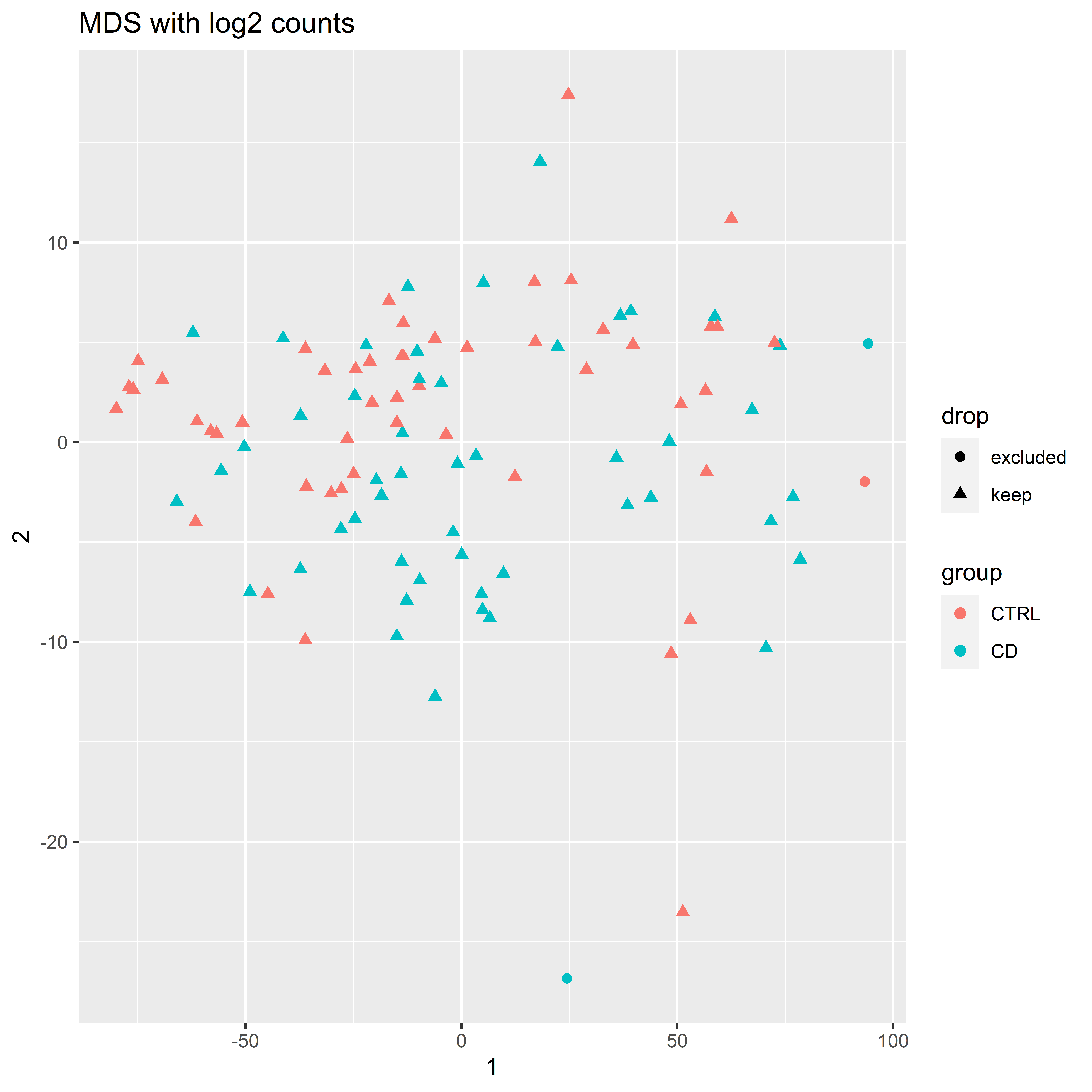
keepSamples = row.names(mds)[! row.names(mds) %in% excl]

ddsMat = ddsMat[,keepSamples]

ddsMat = estimateSizeFactors(ddsMat)

distance=dist(log2(t(counts(ddsMat)+1)))

# hierarchical clustering ####

HC = hclust(distance, method = "ward.D2")
plot(HC, main = "clustered samples log2(counts + 1)", cex = 0.4)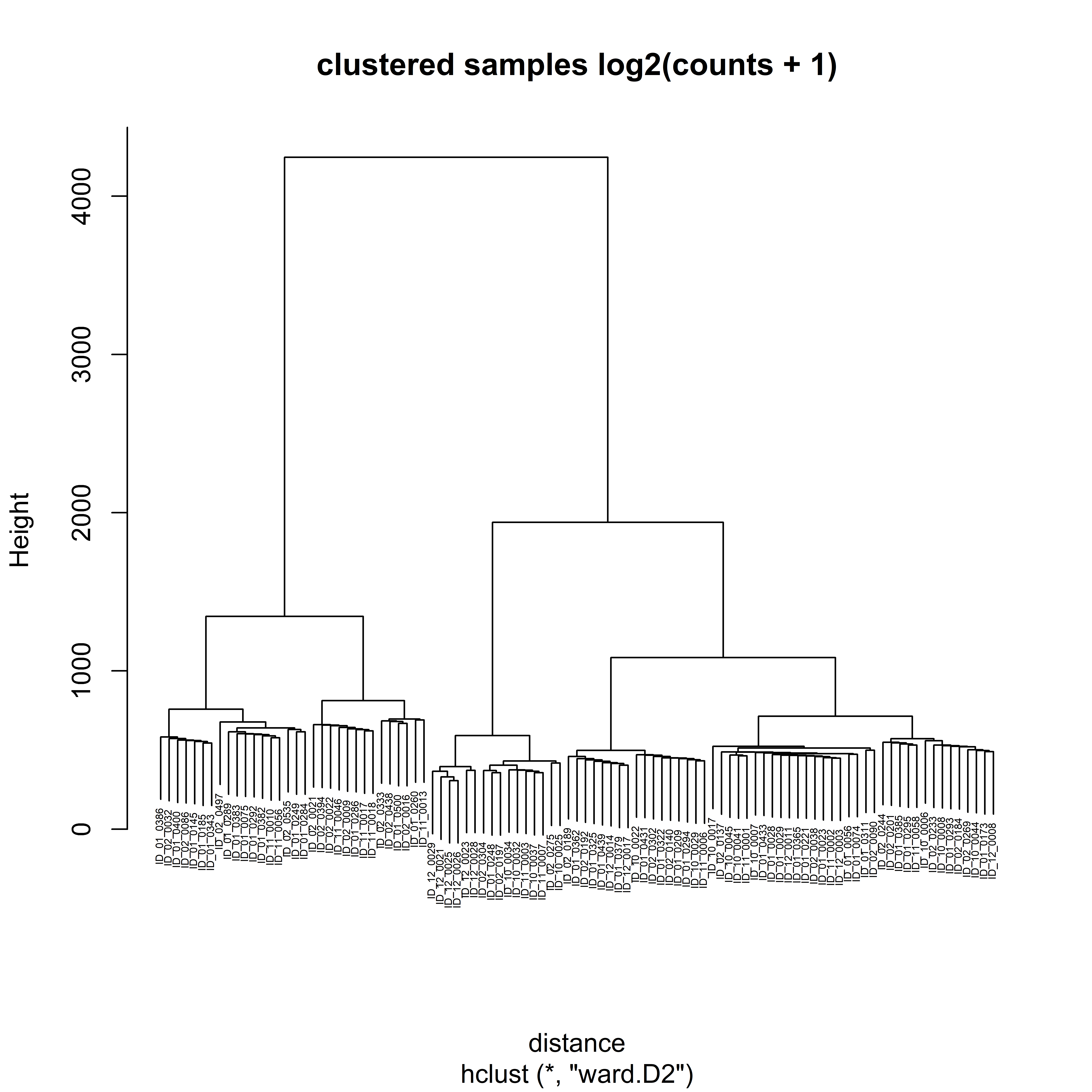
# visual inspection no obvious cluster detectable
n = 2 # check outlier cluster
clusters = cutree(HC,k = n)
tab=table(clusters)

# drop if a cluster hols only 5 percent of the cohort
keeper=as.numeric(names(tab)[tab>0.05*length(clusters)])

keepSamples = names(clusters[clusters %in% keeper])
dds_filt = ddsMat[,keepSamples]
dds_filt = estimateSizeFactors(dds_filt)
replot cleaned samples
# replot with normalized and cleaned data
cpm = counts(dds_filt, normalized = T)
log2_cpm = log2(cpm+1)

distance = dist(t(log2_cpm))
sampleDistMatrix <- as.matrix(distance)

rownames(sampleDistMatrix) <- rownames(colData(dds_filt))
colnames(sampleDistMatrix) <- rownames(colData(dds_filt))
colors <- colorRampPalette( rev(brewer.pal(9, "Blues")) )(255)


ann_colors = list(
  group = groupcol,
  contraceptives = ccptcol,
  site = sitecol)

pheatmap(sampleDistMatrix,
         clustering_distance_rows = distance,
         clustering_distance_cols = distance,
         clustering_method = "ward.D2",
         border_color = NA,
         annotation_row = Patdata[,c("Age", "site", "X260_280", "Timediff_ExtrPurification")],
         annotation_col = Patdata[,c("group", "scrsympt",clinFact[-c(1,2)])],
         col = colors,
         annotation_colors = ann_colors,
         main = "Distances normalized log2 counts, after filtering")
Samples Excluded: 01-0515, 02-0211, 02-0354
Surrogate variable analysis
# only tags with enough reads
idx1  <- rowMeans(cpm) > 1
sd = apply(log2_cpm, 1, sd)

# only tags with some variance
idx2 = sd> 0.5

cpm_subset = cpm[idx1 & idx2,]

mod  <- model.matrix(designh1, colData(dds_filt))
mod0 <- model.matrix(designh0, colData(dds_filt))

nsv = num.sv(cpm_subset, mod, method = "be")

svaset <- svaseq(cpm_subset, mod, mod0, n.sv = nsv)
Number of significant surrogate variables is: 32
Iteration (out of 5 ):1 2 3 4 5 Patdata = cbind(colData(dds_filt), as.data.frame(svaset$sv))
colData(dds_filt) <- Patdata
save(dds_filt, file= paste0(Home,"/output/ProcessedData.RData"))Total Number of Surrogate Variables extracted: 32
Sample statistics after cleaning
Patreads = colSums(cpm)

dds_filt$reads_per_sample_cleaned = Patreads

clPatdata = as.data.frame(colData(dds_filt))

res = table_sumstat(clPatdata,
                    columns=unique(c(tablevariates, clinFact,modelFact, envFact, genomicvariates)),
                    groupfactor = "group")
Warning in chisq.test(xx, correct = FALSE): Chi-squared approximation may be
incorrect
Warning in chisq.test(xx, correct = FALSE): Chi-squared approximation may be
incorrectWarning: glm.fit: fitted probabilities numerically 0 or 1 occurredres
--------Summary descriptives table by 'group'---------

________________________________________________________________________
                                 CTRL               CD         p.overall
                                 N=50              N=49
¯¯¯¯¯¯¯¯¯¯¯¯¯¯¯¯¯¯¯¯¯¯¯¯¯¯¯¯¯¯¯¯¯¯¯¯¯¯¯¯¯¯¯¯¯¯¯¯¯¯¯¯¯¯¯¯¯¯¯¯¯¯¯¯¯¯¯¯¯¯¯¯
site:                                                            0.164
    FRA                       24 (48.0%)        13 (26.5%)
    AAC                       9 (18.0%)         17 (34.7%)
    BCN                       5 (10.0%)          8 (16.3%)
    BLB                       6 (12.0%)          6 (12.2%)
    SZG                       6 (12.0%)          5 (10.2%)
Age                          16.1 (1.60)        15.8 (1.49)      0.404
tsympt                       0.00 (0.00)        4.76 (2.50)     <0.001
Pubstat:                                                         0.170
    Latepubertal              35 (70.0%)        41 (83.7%)
    Postpubertal              15 (30.0%)         8 (16.3%)
cigday_1                     0.52 (2.08)        6.14 (6.57)     <0.001
contraceptives:                                                  0.025
    no                        40 (80.0%)        28 (57.1%)
    yes                       10 (20.0%)        21 (42.9%)
PC_1                         0.00 (0.02)        0.00 (0.02)      0.575
PC_2                         -0.01 (0.01)       0.00 (0.02)      0.010
PC_3                         0.00 (0.01)        0.00 (0.03)      0.667
PC_4                         0.00 (0.02)        0.00 (0.02)      0.828
int_dis:                                                        <0.001
    no                        45 (90.0%)        20 (40.8%)
    yes                       5 (10.0%)         29 (59.2%)
medication:                                                      0.001
    no                        47 (94.0%)        32 (65.3%)
    yes                       3 (6.00%)         17 (34.7%)
Matsmk:                                                          0.071
    no                        39 (81.2%)        24 (61.5%)
    yes                       9 (18.8%)         15 (38.5%)
Matagg:                                                          0.001
    no                        47 (97.9%)        30 (71.4%)
    yes                       1 (2.08%)         12 (28.6%)
FamScore                     0.20 (0.49)        0.76 (0.80)     <0.001
EduPar                       8.11 (2.66)        5.94 (2.62)     <0.001
n_trauma                     0.86 (1.11)        2.16 (1.83)     <0.001
X260_280                     1.84 (0.02)        1.84 (0.02)      0.748
ng_per_ul                     642 (252)          731 (299)       0.113
Timediff_ExtrPurification    4.34 (3.01)        4.02 (3.38)      0.620
reads_per_sample          11017072 (5505663) 9475335 (4256539)   0.122
¯¯¯¯¯¯¯¯¯¯¯¯¯¯¯¯¯¯¯¯¯¯¯¯¯¯¯¯¯¯¯¯¯¯¯¯¯¯¯¯¯¯¯¯¯¯¯¯¯¯¯¯¯¯¯¯¯¯¯¯¯¯¯¯¯¯¯¯¯¯¯¯
setwd(tempdir())
export2word(res, file = paste0(Home,"/output/table1_filtered.docx"))
setwd(Home)- Total number of samples: 99
- Total number of Tags: 216 102
- Tags in TFbinding sites: 114 671
- Tags in CpGs:
Var1 Freq cpg 66346 NoCpg 149756 - Tags per feature
Var1 Freq downstream 7177 exonic 19002 intronic 133566 splicing 624 upstream 37979 UTR3 4885 UTR5 12869
sessionInfo()R version 4.0.3 (2020-10-10)
Platform: x86_64-w64-mingw32/x64 (64-bit)
Running under: Windows 10 x64 (build 19042)
Matrix products: default
locale:
[1] LC_COLLATE=German_Germany.1252 LC_CTYPE=German_Germany.1252
[3] LC_MONETARY=German_Germany.1252 LC_NUMERIC=C
[5] LC_TIME=German_Germany.1252
attached base packages:
[1] parallel stats4 stats graphics grDevices utils datasets
[8] methods base
other attached packages:
[1] scales_1.1.1 RCircos_1.2.1
[3] compareGroups_4.4.6 cluster_2.1.0
[5] kableExtra_1.3.1 knitr_1.30
[7] glmpca_0.2.0 sva_3.38.0
[9] BiocParallel_1.24.1 genefilter_1.72.0
[11] mgcv_1.8-33 nlme_3.1-151
[13] pheatmap_1.0.12 vsn_3.58.0
[15] DESeq2_1.30.0 SummarizedExperiment_1.20.0
[17] Biobase_2.50.0 MatrixGenerics_1.2.0
[19] matrixStats_0.57.0 GenomicRanges_1.42.0
[21] GenomeInfoDb_1.26.2 IRanges_2.24.1
[23] S4Vectors_0.28.1 BiocGenerics_0.36.0
[25] forcats_0.5.0 stringr_1.4.0
[27] dplyr_1.0.2 purrr_0.3.4
[29] readr_1.4.0 tidyr_1.1.2
[31] tibble_3.0.4 tidyverse_1.3.0
[33] corrplot_0.84 ggplot2_3.3.3
[35] gplots_3.1.1 RColorBrewer_1.1-2
[37] data.table_1.13.6 workflowr_1.6.2
loaded via a namespace (and not attached):
[1] uuid_0.1-4 readxl_1.3.1 backports_1.2.0
[4] systemfonts_0.3.2 splines_4.0.3 digest_0.6.27
[7] htmltools_0.5.1.1 fansi_0.4.1 magrittr_2.0.1
[10] Rsolnp_1.16 memoise_2.0.0 limma_3.46.0
[13] annotate_1.68.0 modelr_0.1.8 officer_0.3.16
[16] colorspace_2.0-0 blob_1.2.1 rvest_0.3.6
[19] haven_2.3.1 xfun_0.20 crayon_1.3.4
[22] RCurl_1.98-1.2 jsonlite_1.7.2 survival_3.2-7
[25] glue_1.4.2 gtable_0.3.0 zlibbioc_1.36.0
[28] XVector_0.30.0 webshot_0.5.2 DelayedArray_0.16.0
[31] DBI_1.1.1 edgeR_3.32.1 Rcpp_1.0.5
[34] viridisLite_0.3.0 xtable_1.8-4 bit_4.0.4
[37] preprocessCore_1.52.1 truncnorm_1.0-8 httr_1.4.2
[40] ellipsis_0.3.1 mice_3.12.0 farver_2.0.3
[43] pkgconfig_2.0.3 XML_3.99-0.5 dbplyr_2.0.0
[46] locfit_1.5-9.4 labeling_0.4.2 tidyselect_1.1.0
[49] rlang_0.4.10 later_1.1.0.1 AnnotationDbi_1.52.0
[52] munsell_0.5.0 cellranger_1.1.0 tools_4.0.3
[55] cachem_1.0.1 cli_2.2.0 generics_0.1.0
[58] RSQLite_2.2.2 broom_0.7.3 evaluate_0.14
[61] fastmap_1.1.0 yaml_2.2.1 bit64_4.0.5
[64] fs_1.5.0 zip_2.1.1 caTools_1.18.1
[67] whisker_0.4 xml2_1.3.2 compiler_4.0.3
[70] rstudioapi_0.13 affyio_1.60.0 reprex_1.0.0
[73] geneplotter_1.68.0 stringi_1.5.3 HardyWeinberg_1.7.1
[76] highr_0.8 ps_1.5.0 gdtools_0.2.3
[79] lattice_0.20-41 Matrix_1.2-18 vctrs_0.3.6
[82] pillar_1.4.7 lifecycle_0.2.0 BiocManager_1.30.10
[85] flextable_0.6.2 bitops_1.0-6 httpuv_1.5.5
[88] R6_2.5.0 affy_1.68.0 promises_1.1.1
[91] KernSmooth_2.23-18 writexl_1.3.1 MASS_7.3-53
[94] gtools_3.8.2 assertthat_0.2.1 chron_2.3-56
[97] rprojroot_2.0.2 withr_2.4.1 GenomeInfoDbData_1.2.4
[100] hms_1.0.0 grid_4.0.3 rmarkdown_2.6
[103] git2r_0.28.0 base64enc_0.1-3 lubridate_1.7.9.2